09. When related coins drifted apart
Residuals, hedge ratios, sizing, and a recent DRY campaign with a narrower purpose.
Investing on my own · Part 9/22 · Evidence through 2026-09-22. Historical research is distinct from DRY and live execution.
If two coins usually move together and suddenly diverge, will they come back together? That was the starting question for my statistical-arbitrage work.
Unlike a factor that ranks a large universe, this approach focuses on relationships between assets. I wanted to know whether one coin had become unusually expensive even after accounting for the broader market move.
⚖️ More than subtracting two prices
Imagine, purely as an example, that A trades at 100 and B at 50. One unit of A and two units of B have usually moved together. If A rises to 110 while B stays at 50, a possible trade is to short A and buy B.
Past co-movement is not a guarantee of convergence. A may have received genuinely good news. The expensive side might keep rising instead of the cheap side catching up.
I explored residuals after removing common market movements, hedge ratios that change over time, and longer-run relationships across several assets. A residual is simply the part of a price move that the estimated relationship does not explain.
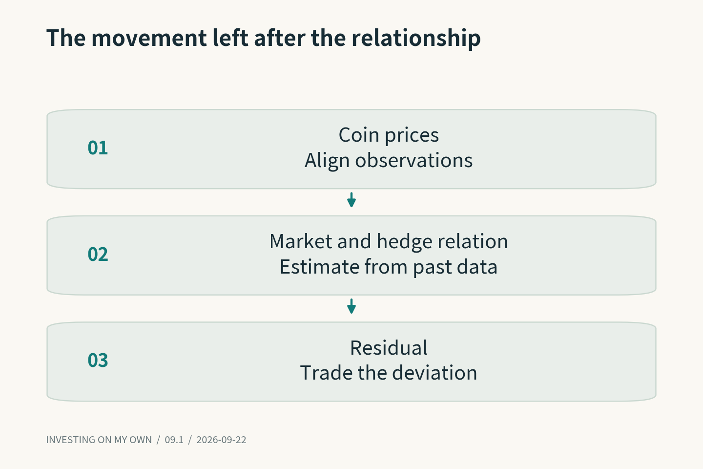
Kalman-based models allowed the relationship to evolve gradually. Johansen-based work searched for relatively stable combinations of multiple price series. The model names mattered less to execution than the resulting instructions: which assets to buy or sell, and in what quantities.
I also distinguished a large current deviation from a forecast that the deviation would narrow. Those are related but different signals. A model trained to predict a seven-day outcome does not automatically answer a two-hour trading question.
📈 Larger positions changed the results
The September follow-up separated the 2022–2024 evaluation from already-observed 2025 outcomes. The longer history used in model construction was not interchangeable with the performance window below. In particular, Johansen’s starting value in 2022 carried forward positions and equity from the preceding year; it was not a fresh account opened that day.
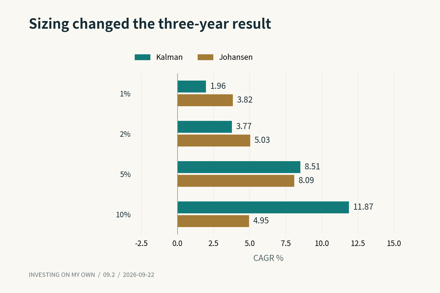
For the Kalman family, position sizes of 1%, 2%, 5%, and 10% produced 2022–2024 compound annual growth rates of 1.96%, 3.77%, 8.51%, and 11.87%. The corresponding Johansen results were 3.82%, 5.03%, 8.09%, and 4.95%.
Johansen performance fell when sizing increased from 5% to 10%. Doubling position size did not double the outcome. Capital constraints and overlapping opportunities changed what the portfolio could actually hold.
For 2025, Kalman total returns at those same sizes were 14.82%, 30.19%, 56.24%, and 78.42%. Johansen returned 3.56%, 6.76%, 11.90%, and 25.30%. These were follow-up results from an observed period, not a newly opened untouched holdout.
I also revisited delisting treatment. A data file may retain a price after trading volume disappears. That does not establish that an order could have exited there. A single untradeable component can change the economics of an otherwise balanced basket.
A favorable chart therefore did not settle the implementation question. I still needed valid quantity increments, minimum order sizes, funding treatment, and a check on the market exposure left by the full basket.
🧪 A recent DRY test asked a narrower question
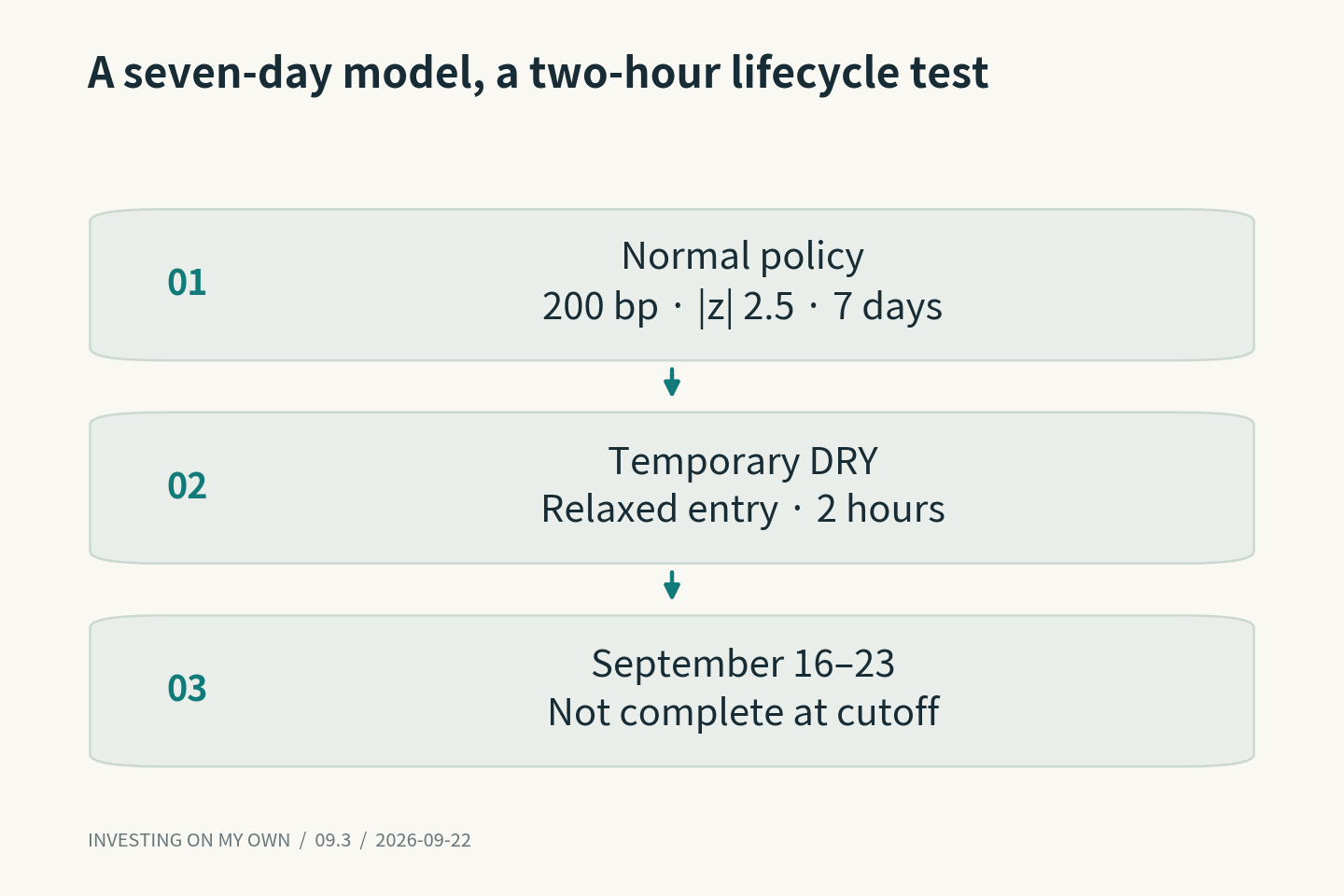
On September 16, I started a separate seven-day DRY campaign. It recorded simulated fills against public quotes rather than placing real-money exchange orders. Its scheduled end was September 23, after this series’ September 22 evidence cutoff.
It would be inaccurate to describe that week as completed at the cutoff. It would also be inaccurate to present the campaign as a direct reproduction of the normal strategy.
The normal policy required a 200-basis-point net edge, a standardized deviation of 2.5, and a seven-day holding period. The test relaxed entry conditions and shortened holding to two hours so that the execution lifecycle could be observed.
The underlying forecast model remained a seven-day model. Two-hour trade outcomes could not be used as a clean evaluation of its original forecast horizon. The campaign primarily examined whether entry, holding, exit, funding, and ledger records connected correctly in actual elapsed time.
The start record contained two simulated fills based on public quotes, one for each side. Those were not exchange confirmations of real orders. The activation record also distinguished this narrow test from restarting the shared engine or changing REAL settings; neither was done for that activation.
The September 22 review conversation also identified a model input still being sought at its old path after archival. A successful launch did not establish uninterrupted signal readiness throughout the campaign. The launch and the later problem both belonged in the account.
These distinctions make the description less tidy than a single performance headline. They are still necessary. A historical portfolio return, a successful simulated order lifecycle, and a live trading return are different observations.
I originally cared most about whether the two prices moved closer together. More recently, I have been asking whether both positions can be maintained until that happens, and what the system should do if only one side remains.
The phrase “statistical arbitrage” sounds like a category with a clear boundary. An actual inventory of open positions asks much more specific questions. That is where this research has moved: from an estimated relationship toward a testable account of how the relationship would be traded.
Previous · Series index · Next